A few months ago, I did my first 3D reconstruction of a house using the Tricopter V2.5 and my GoPro Hero 3 Black. Thanks to my friend Thibault, for letting me experiment this on his house!
In this post we will see how the 3D reconstruction is performed from the GoPro pictures. After what I will present some applications such as:
- measuring distances, areas and volumes in the model;
- building orthophotos and digital elevation models;
- displaying the 3D model in Google Earth.
The 3D reconstruction
The 3D reconstruction has been done by photogrammetry using the software Agisoft PhotoScan. They are many other photogrammetry softwares on the market, such as Pix4D which works similarly to PhotoScan.
Photogrammetry method consists of computing the 3D model of a scene from 2D images captured from different viewpoints. The captured images have to overlap. It means that each part of the scene you want to reconstruct must appear in multiple images. By matching the corresponding pixels in the images, the 3D positions of the corresponding points are obtained by triangulation and by performing global optimization. In the process, the camera locations (from where the images have been captured) and the camera intrinsic parameters (such as the distortion profile) are computed to minimize the quadratic error of 3D point reprojections over all the images. After what, a mesh and a texture are computed from the 3D point cloud and the images, providing the final result.
Let’s now see how it works in practice.
As I explained, the first step is to capture pictures of the house from various angles. I flew the drone around the house while the GoPro 3 was taking a 12 Megapixel picture every second.
The GoPro isn’t the best camera for this application:
- It has a fisheye lens which provides high distortion and reduces the sharpness in the corner;
- It uses rolling shutter speed (as with any CMOS sensors, images are captured line by line) and the image can be distorted if the drone moves fast;
- The automatic exposure can provide over exposed images which will lack texture (and then lack information to match pixels and build the 3D model);
- The JPEG compression which adds noise (artifacts) in the edges. It would be better to use raw images (which is now possible with the recently released GoPro 5).
But the advantage of the GoPro is to be well suited for use on a drone (small and light weight) and as you will see, the 3D reconstruction accuracy is acceptable.
Here is a sample of the 143 pictures taken from the drone:
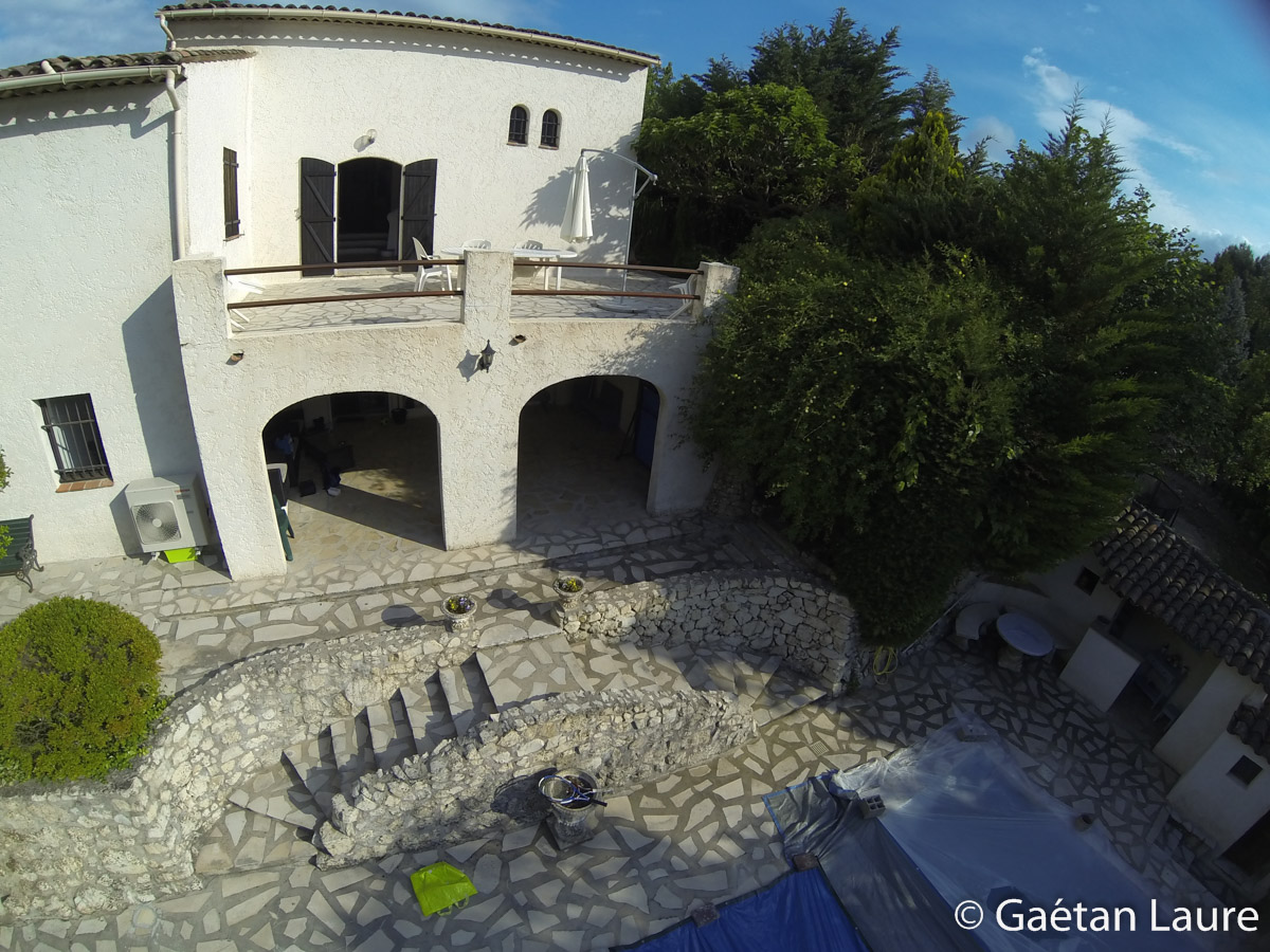
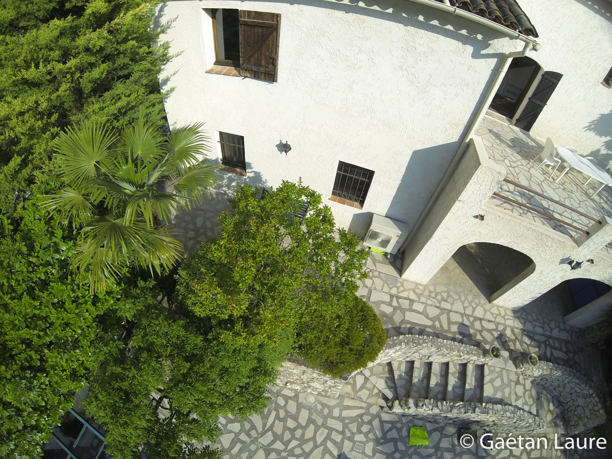
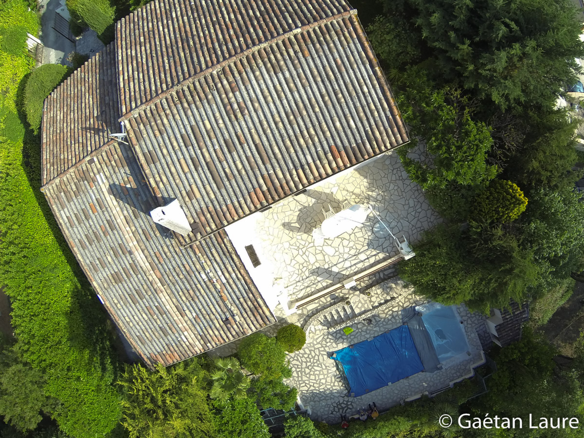
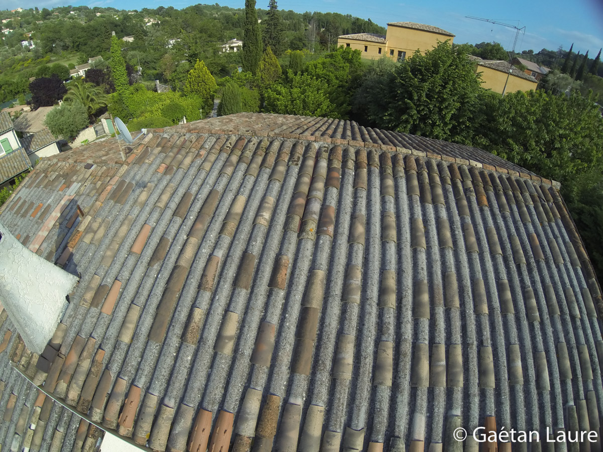
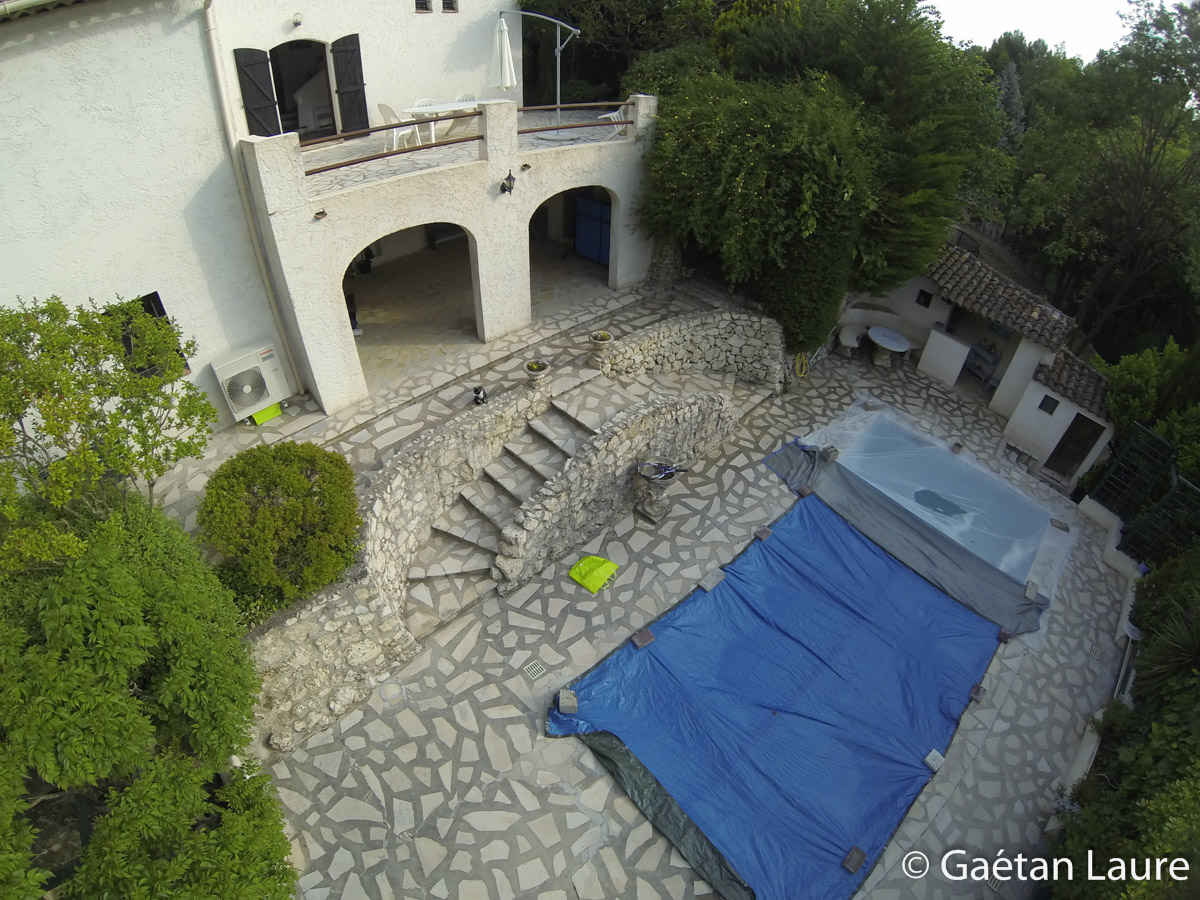
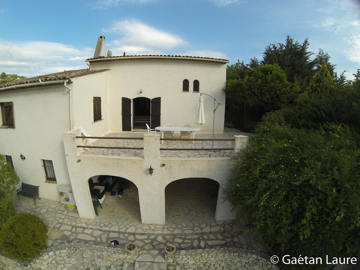
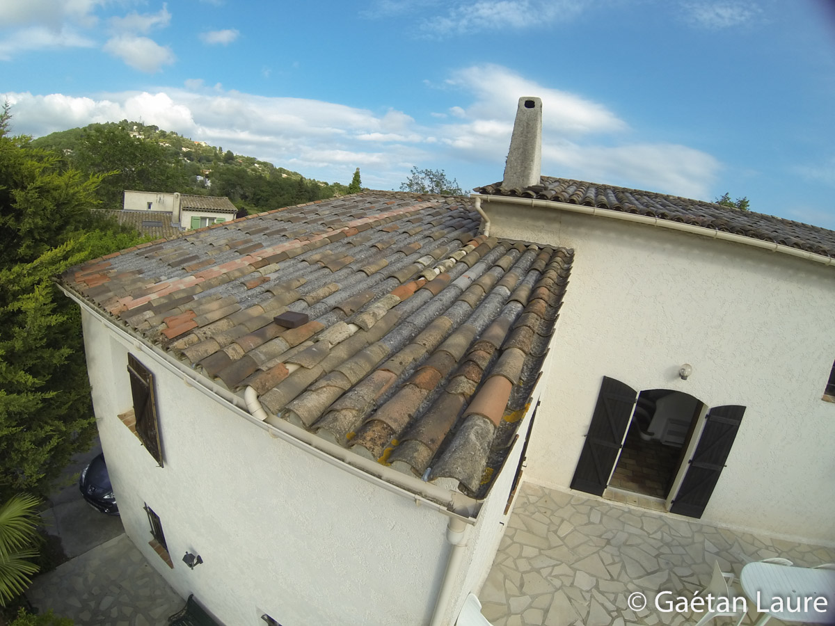
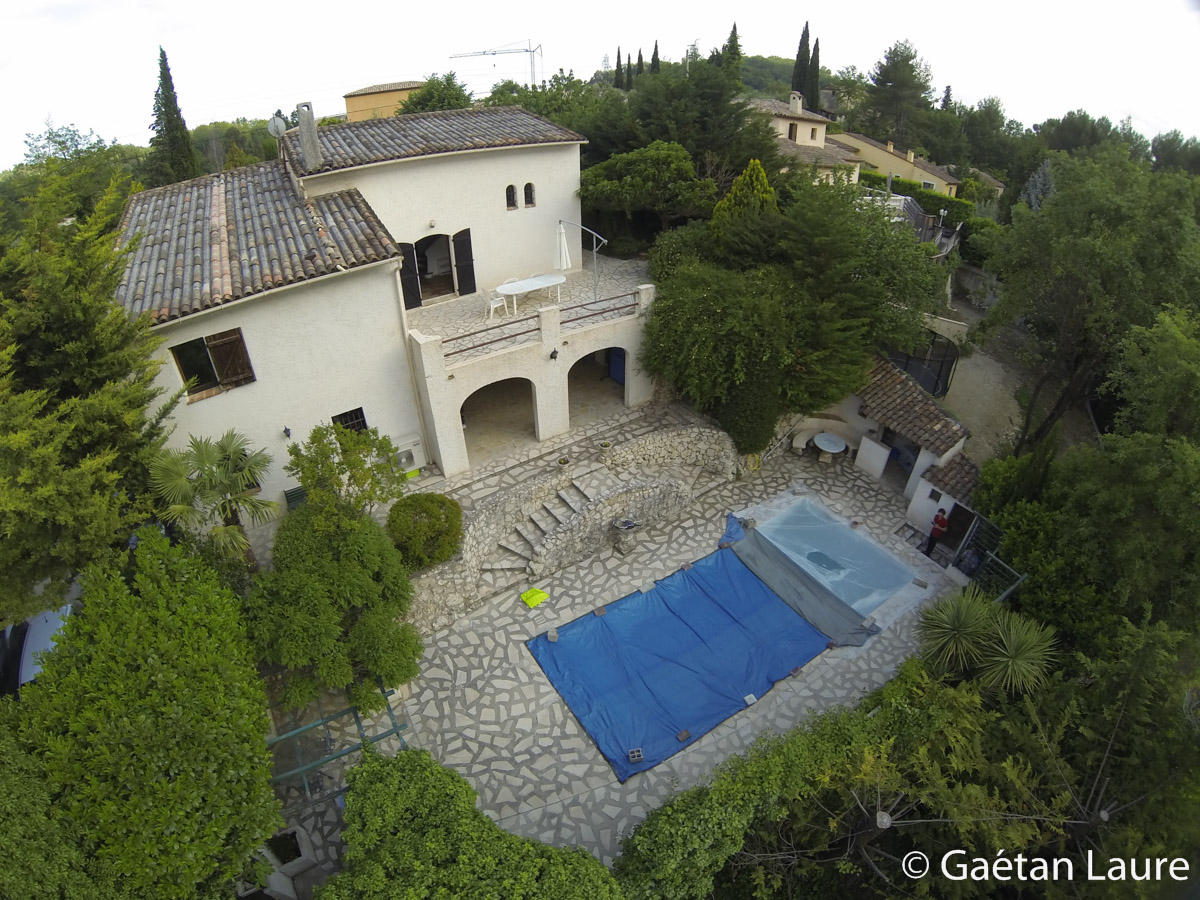
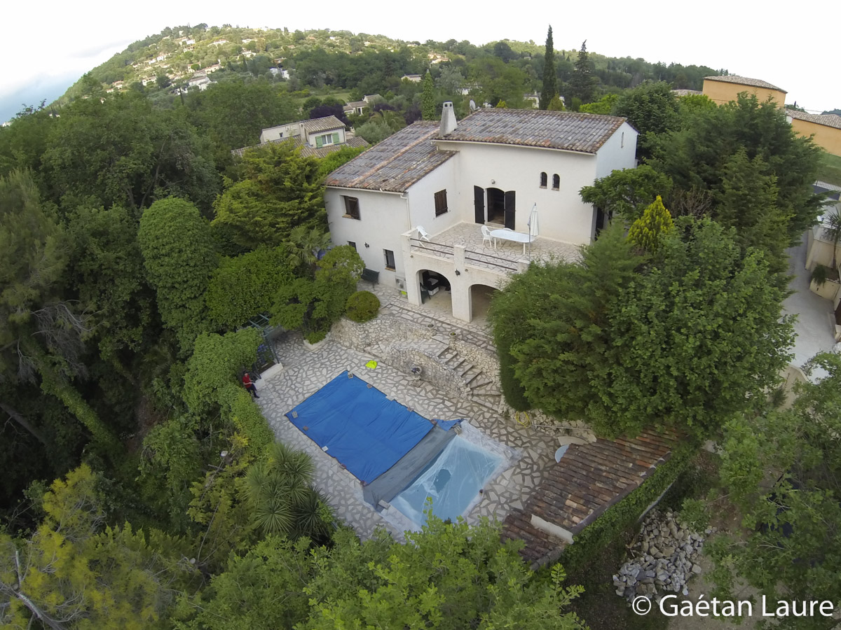
For this test, I mainly took pictures from one side and the roof of the house. Thus, the 3D reconstruction will not cover all the sides.
As you can see, the light and shadows are changing between pictures. The clouds were moving fast on that day. For a better 3D reconstruction result, I should have a constant light between the different shots. When shadows are moving between frame, it’s more difficult for the software to match corresponding pixels.
Now let’s process the pictures using PhotoScan.
In order to minimize the processing time, I use a computer with an i7-6700K (quite powerful 4GHz quad-core processor), 16 GB of RAM and images are stored on an SSD.
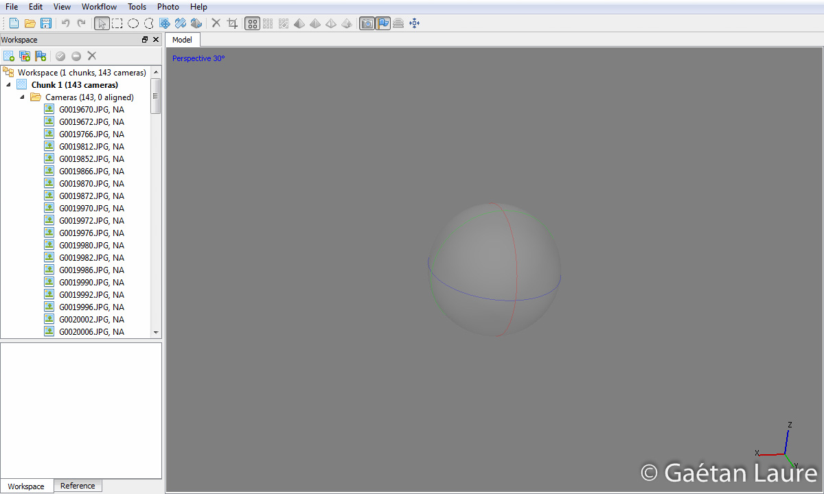
We load the pictures in a new project.
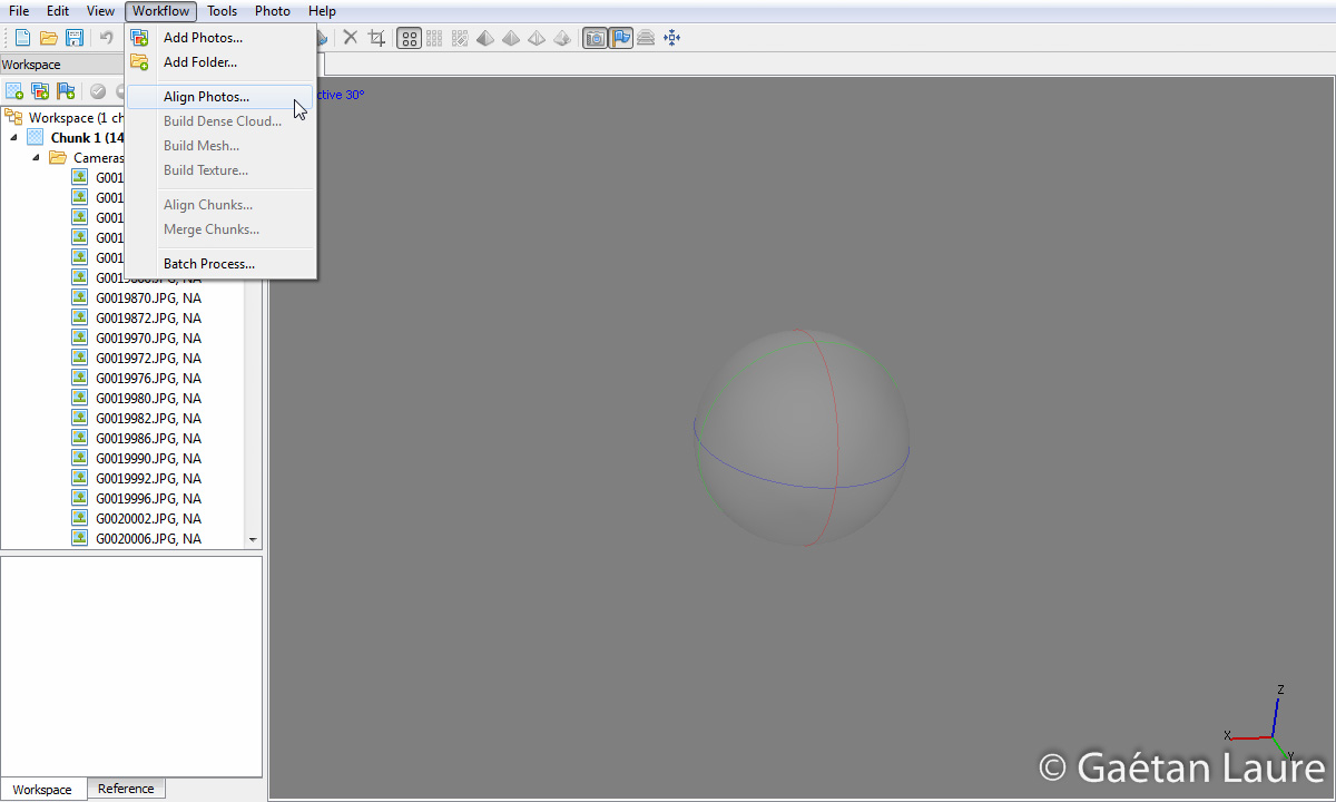
We are going to run all the steps specified in the workflow menu:
- Align Photos;
- Build Dense Cloud;
- Build Mesh;
- Build Texture.

Let’s run the first step to align photos. PhotoScan is going to search for the tie and key points (which are corner points) on each image. After that, it compares the local key points around the tie points to match them (the tie points) between images. A global optimization on all the images will then determine:
- the 3D position of the tie points;
- the position and orientation of the camera for each image;
- the intrinsic parameters of the camera such as the focal length and the distortion model.
In the “Advanced” section, I kept the default parameters: the numbers of key points and tie points found are respectively limited to 40000 and 1000 per image. It’s a good compromise between process time and finding enough tie points to properly align photos.
If the camera positions are initialized using recorded GPS data in the EXIF files, this step will be faster. If you don’t have any GPS information, which was my case, it takes a little longer to process, but works fine as well.

It took 53 mins 40 secs to complete. Images are now aligned and we can see their 3D positions and orientations. We can see from where the photos were taken. I was manually controlling the drone, and tried to move around one side of the house and the roof. The camera was oriented in front, tilted at 45 degrees and tilted down to get all the necessary orientations.
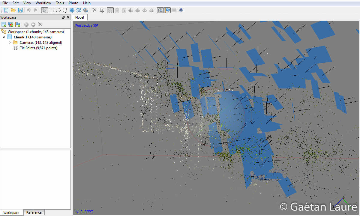
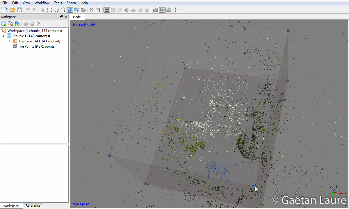
Zooming in. The sparse point cloud represents the tie points used to align photos. We recognize the points used on walls, in white, and the points used on the trees, in green.
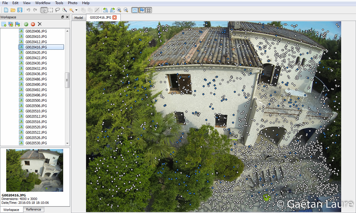
On each image, we can observe the tie points found. Blue ones correspond to used matches (the sparse point cloud). White ones are the tie points which are not used.
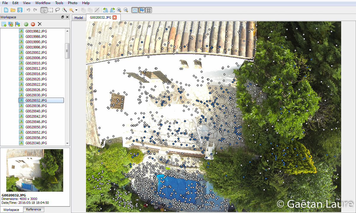
When the walls are over exposed, PhotoScan doesn’t find any tie points on them because of the lack of texture. It then uses other parts of the image such as trees, ground and roof to find tie points. Hopefully it’s not the case of most of the photos. The best configuration would have been to take the photos during a cloudy day, to get a uniform light.

The panel in the menu “Tools -> camera calibration” also provides the camera intrinsic parameters determined during the optimization process.
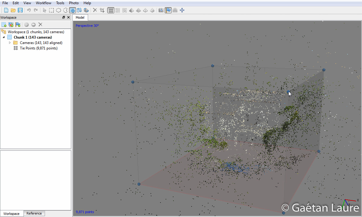
Before computing the dense cloud, the bounding box can be adjusted to limit the reconstruction volume to the house and the garden.
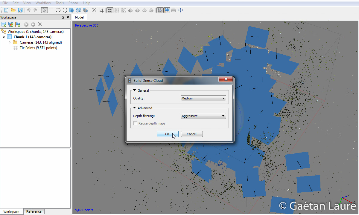
It’s time to compute the dense cloud. During this step, PhotoScan computes the depth information on each image and combines them into one point cloud. To keep the process low time consuming I used the default parameter “medium” for quality. As you will see, it’s enough for the reconstruction of a house. In the “advanced” menu I chose “Aggressive” for “depth filtering” to sort out most of the outliers. It makes sense because there is not too much details in the scene.
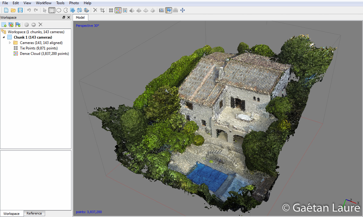
Here is the result! It took 18 mins 31 secs to obtain this dense point cloud representing the house.

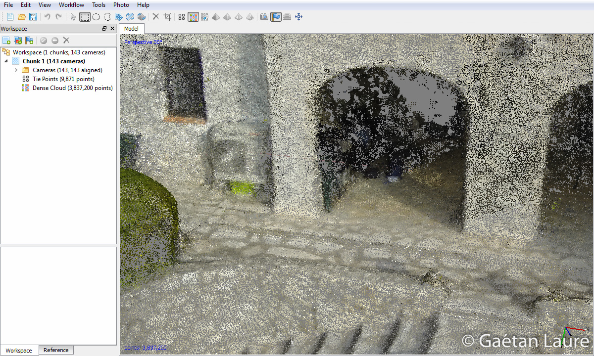
Zooming in.
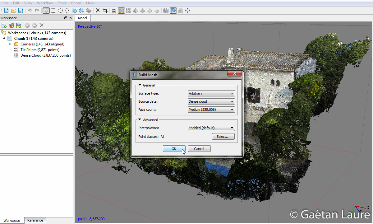
Let’s now run the mesh reconstruction in the workflow menu. I selected again medium parameters, we don’t need too much polygons because most parts of the house are walls and plane surfaces.
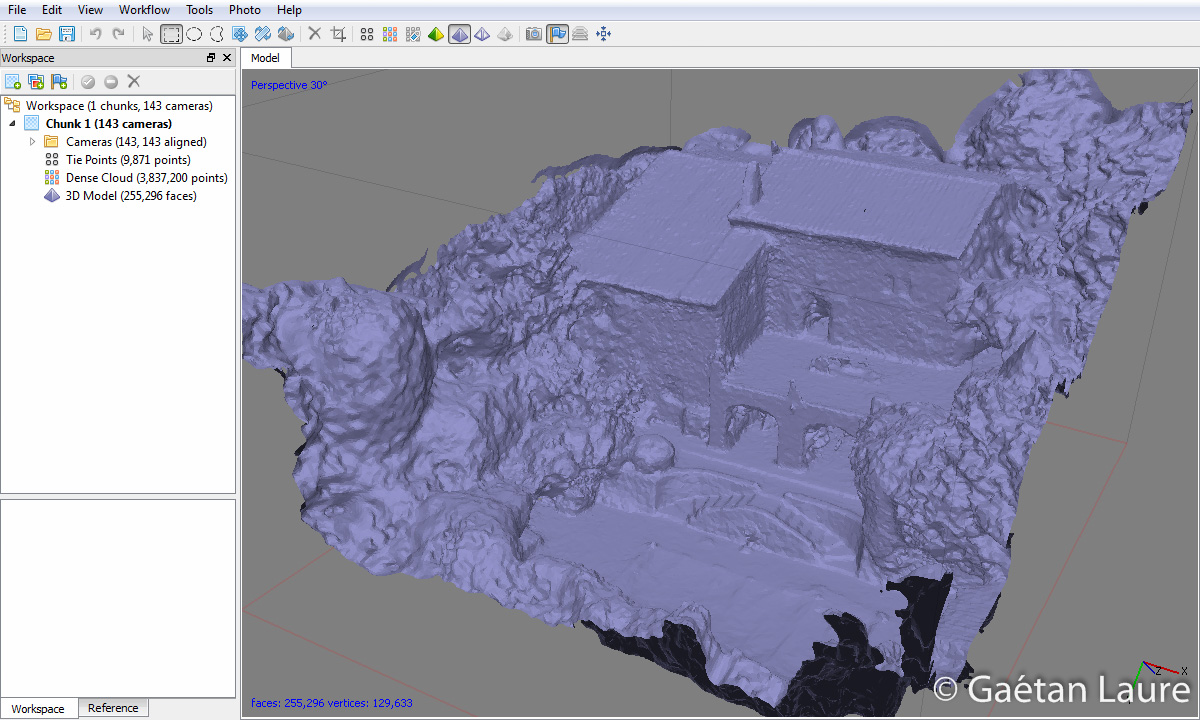
I finally got the 3D mesh of the house, it took 2 mins 54 secs to proceed. We can see that the result is quite good. The walls of the house are not perfectly flat. It may be due to the variation of luminosity between images and overexposed images. Also, as I said before, the GoPro 3 isn’t optimal for 3D reconstruction. It’s mainly due to its fisheye lens inducing distortion that reduces the precision in the corner of images.
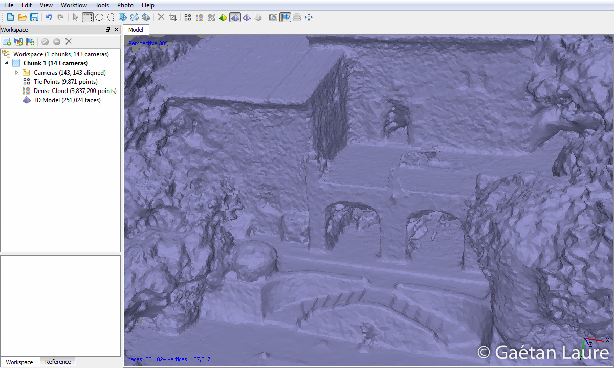
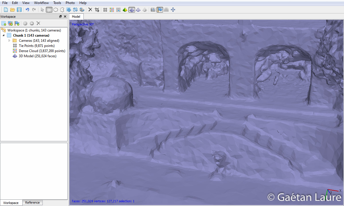
Zooming in.
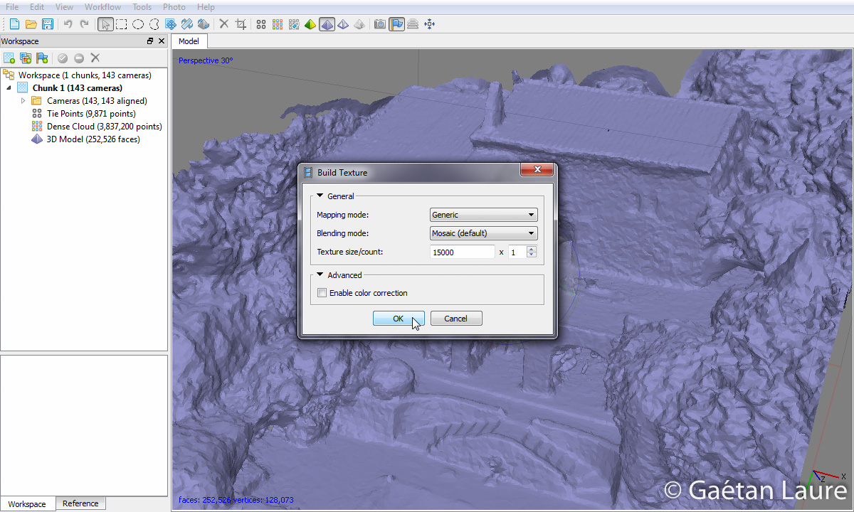
Now the last step is to compute the texture. PhotoScan projects images (and merges them) on the mesh to generate the texture. The size of the texture has a significant effect on the final render. In this case, a 15000×15000 sized texture is optimal (enough details and sufficiently light to be uploaded online).
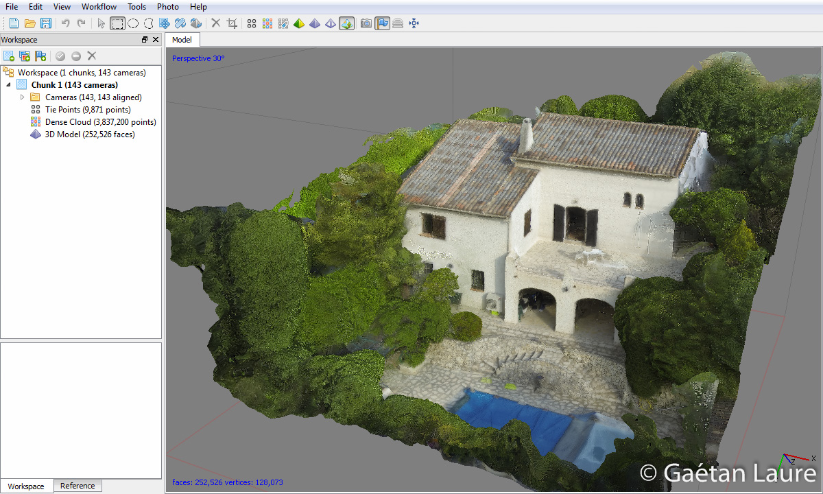
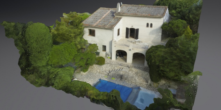
The final result: the mesh with the texture patched on it. It took 2 mins 47 secs to compute the texture.
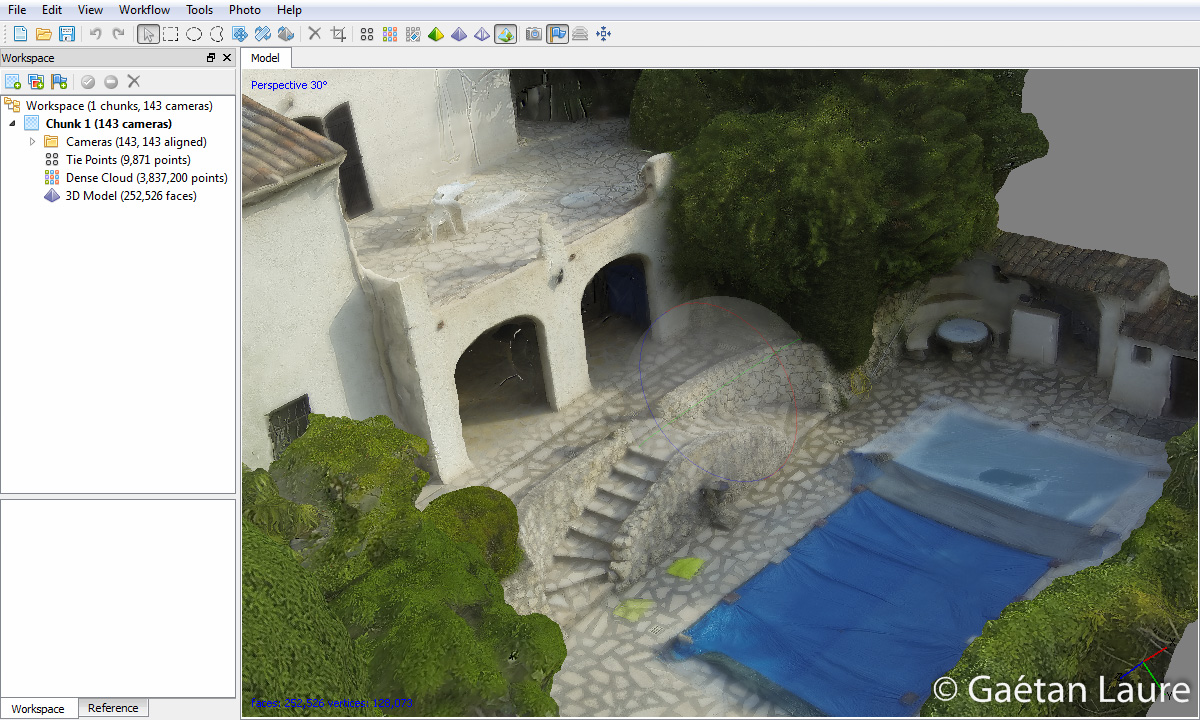
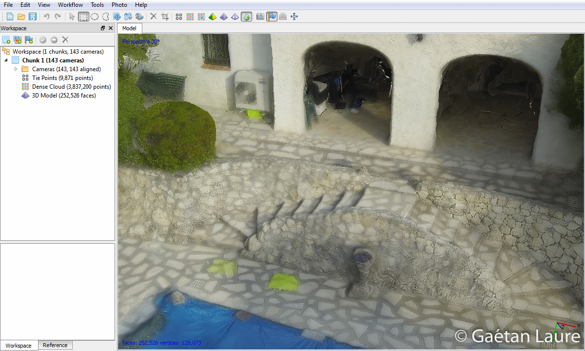
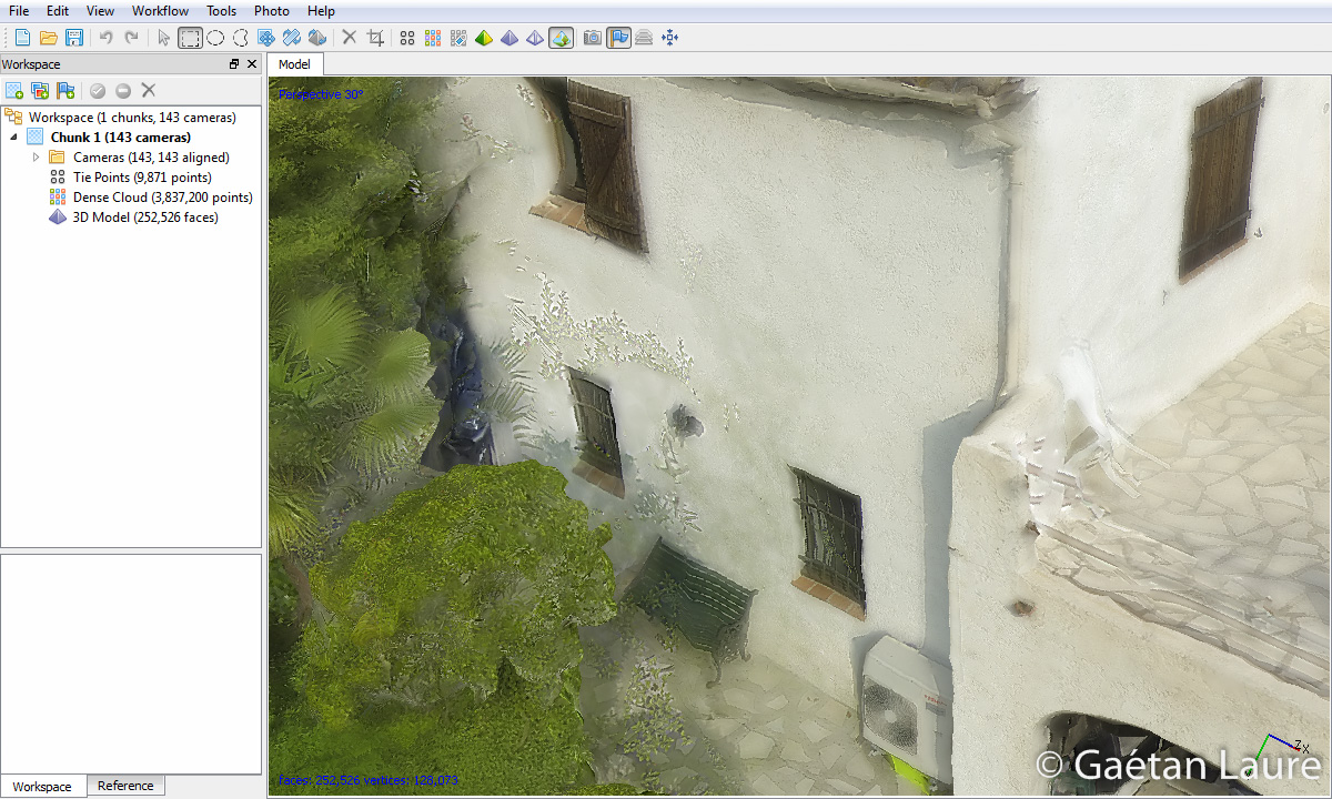
Zooming in, most of the scene is quite good. The texture adds details not represented on the mesh.
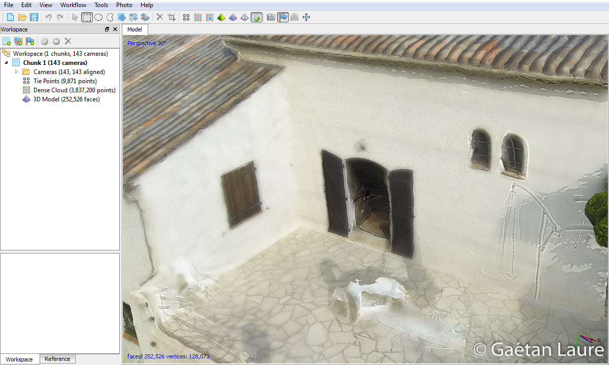
The texture also mask the mesh defects and walls appear flatter.
In some parts where the trees are close to the walls, outlines of the trees have been projected on the house. This can be corrected by editing the texture image.
This is what the texture image looks like (it’s not the original resolution). It’s a 2D image, representing a mosaic of all the house parts. It can be easily edited, to correct defects, as any usual image.

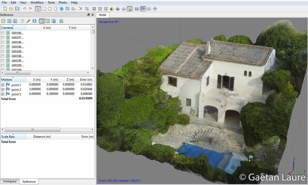
I finally created a local reference coordinate system for this model. For that purpose, I measured two sides of the swimming pool and then defined 3 reference points in the corner of the pool. I provided the coordinates of the three points in the “Markers” table. “Point 1” is used to define the origin, “point 2” the X axis and “point 3” the Y axis of the coordinate system. The “update” button makes PhotoScan perform a short optimization to create the orthogonal coordinate system which fit, with a minimal error, the coordinates provided for the three points. The scale system (in meter) is then also created. After the optimization, the mean error of the three reference points was about 1.5 cm.
The local coordinate system is now correctly defined. The model is then ready to be exported and uploaded online.
The model hosted on Sketchfab. This website works fine using .obj files for the geometry, .mtl files for the material properties and .jpg files for the texture.
Finally it took about 1 hour and 18 mins to compute the 3D model (to process all the workflow steps: align photos, build dense cloud, build mesh and build texture).
Measuring distances, area and volume in the model
Thanks to the local coordinate system, we are now able to measure distances in the model. I compared the measurements of 9 distances in the model to the real corresponding value (classically measured with a tape measure).
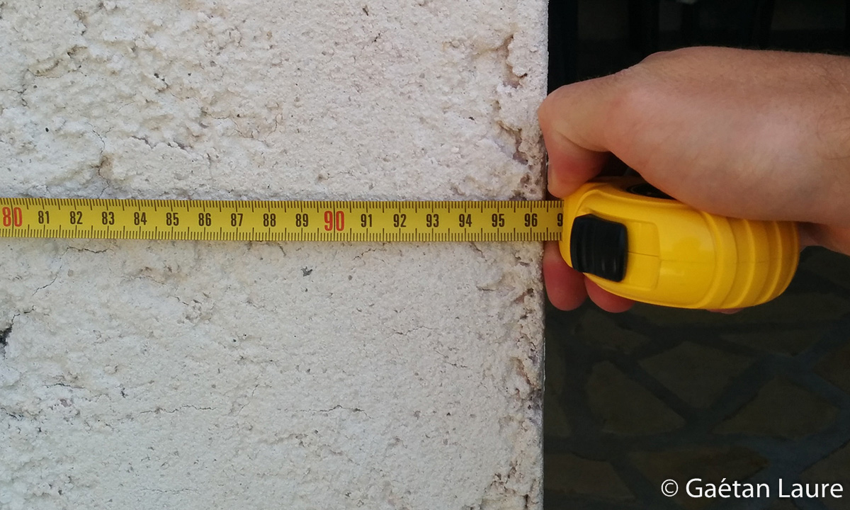

Measuring the real values.
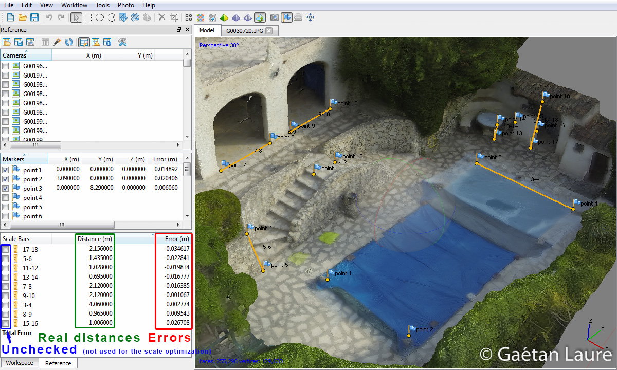
I then created 15 new points to define the 9 distances in the model. We can see them in the “scale bars” panel, but I didn’t use them to scale my model (the purpose here is to check the model accuracy). In the column “Distance (m)” I provided the real measured distances. The column “Error (m)” shows difference between the real measurements and the model measurements. I ordered the distance by error value. We can see that for all the distances, the max error is 3.5 cm (the mean error is 1.96 cm). This result is quite good considering that we used a GoPro, which is not the best camera for this application. Let’s keep in mind that here, errors could come from the model itself, but also from the accuracy with which I located the points to measure distances in the model.
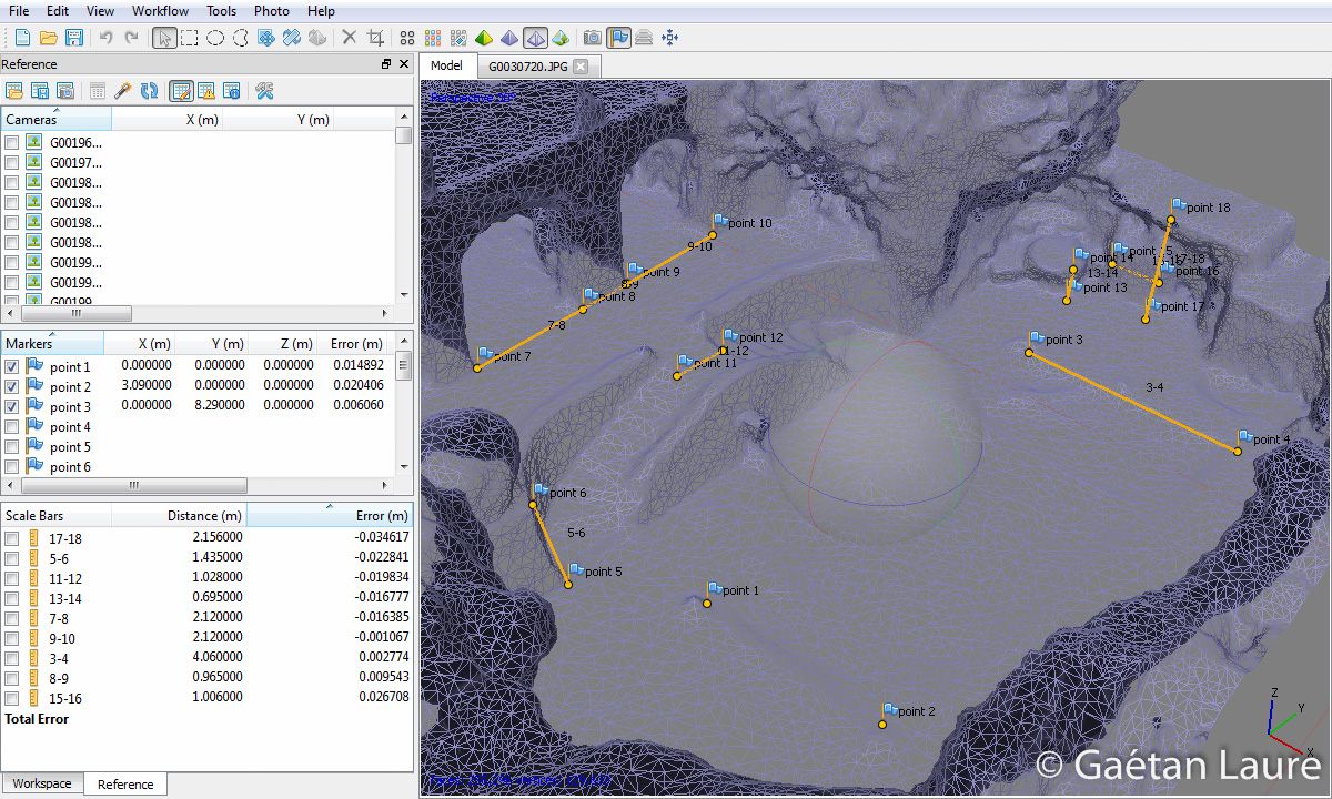
The same distances shown on the wireframe mesh.
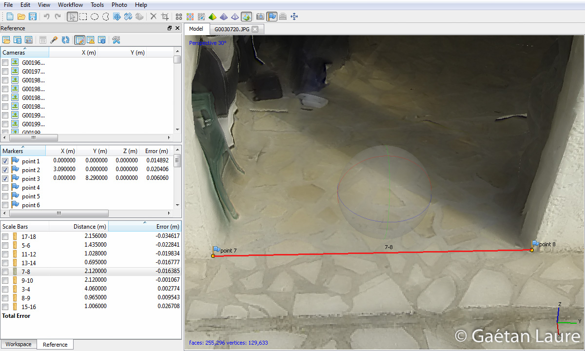
Zoom on the distance 7-8.
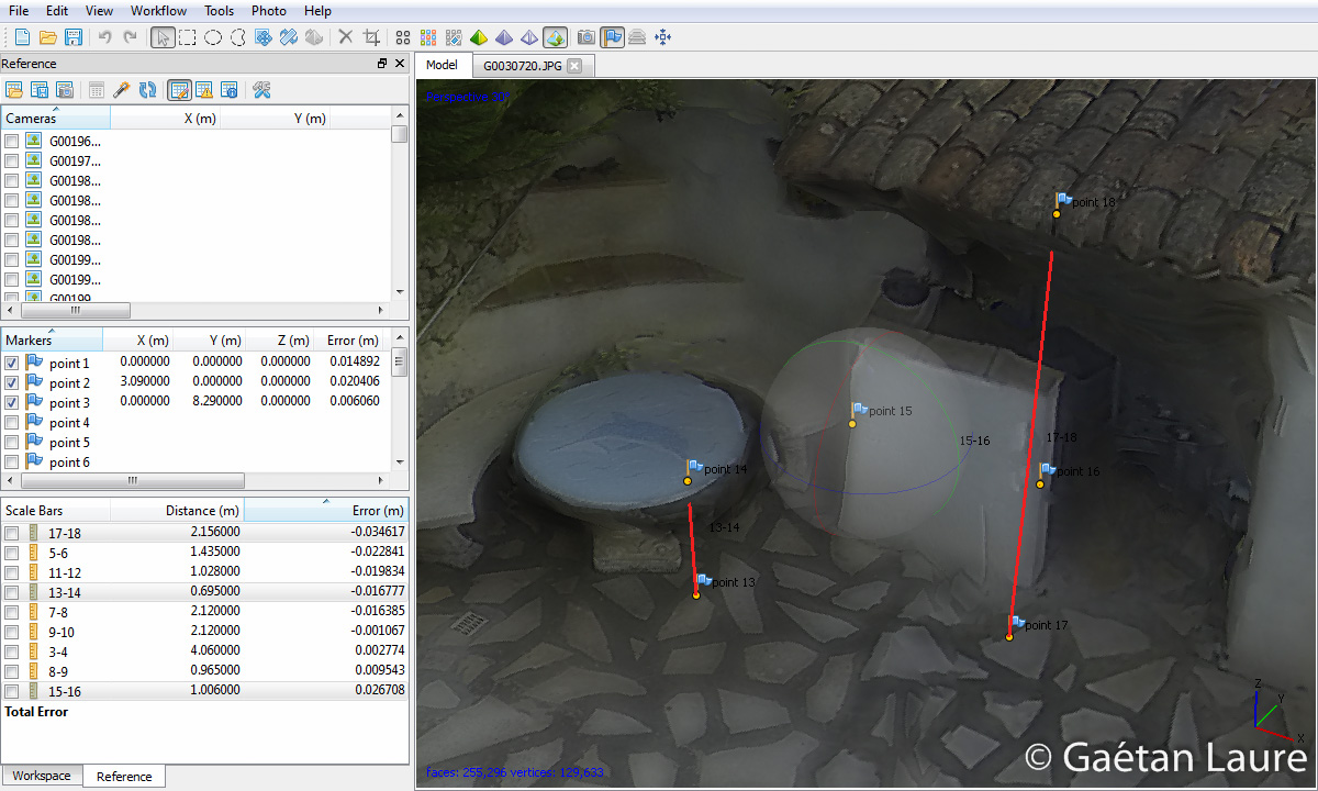
Zoom on the distances 13-14, 15-16 and 17-18.
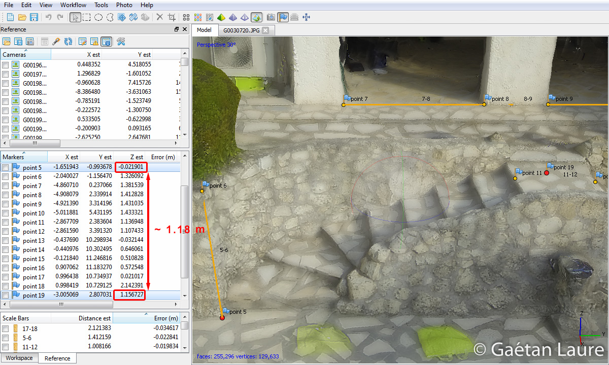
I also measured the height of the 8 steps, between the swimming pool and the house, with the tape measure. Their height are not equal, from 13.1 to 17.6 cm, with an average of 14.5 cm. In the model, the point 19 is estimated 118 cm higher than the point 5 (which is 2 cm close to 8 * 14.5 cm = 116 cm, the height corresponding to the 8 steps).
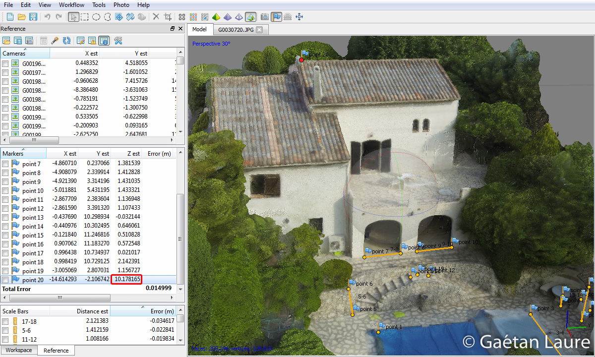
We can also add points to estimate measures that we can’t get with the tape measure. I did it to know the altitude of the top of the house (point 20), the result should be close to 10.18 meters!
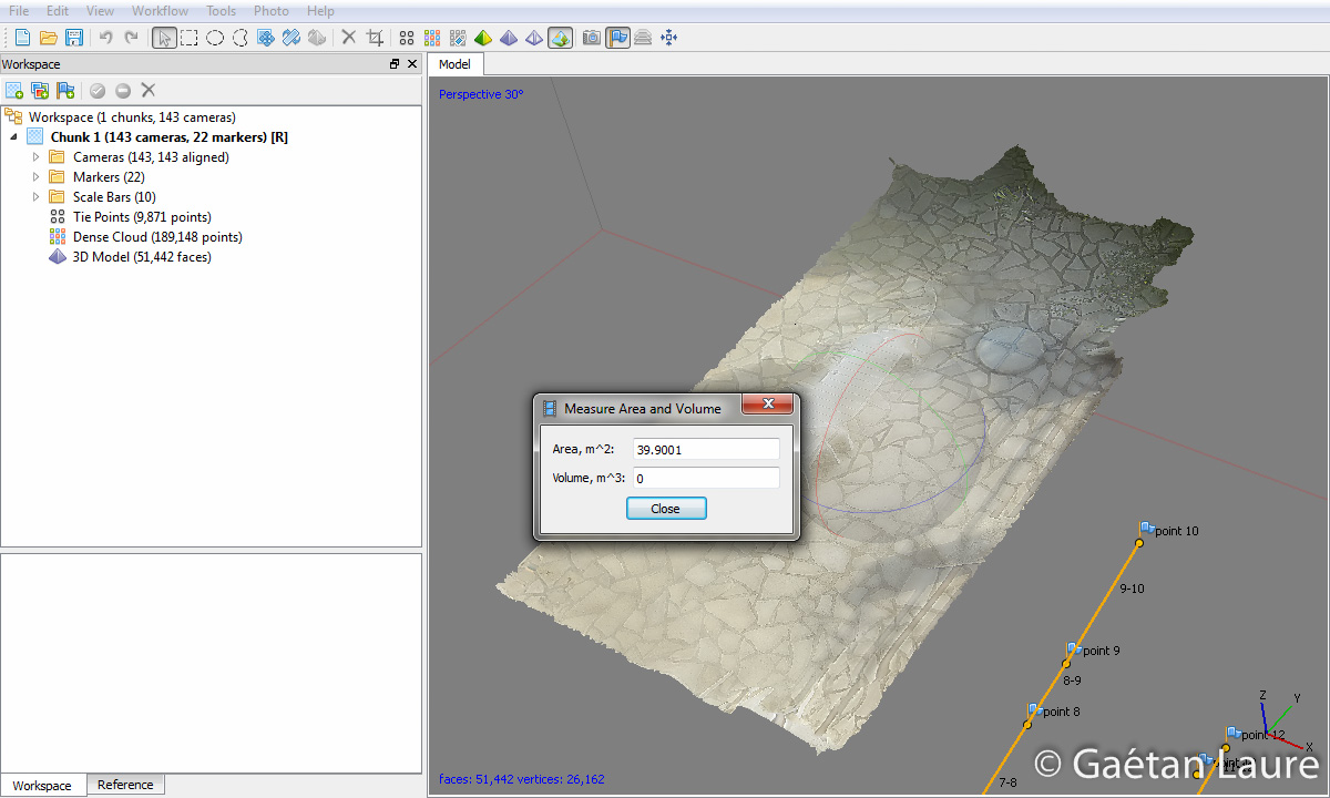
We can also compute areas and volumes directly in PhotoScan. I chose to compute the area of the first floor terrace. I did it restricting the dense point cloud to the terrace and I computed again the mesh (to get a more accurate mesh for this part). Then the area is provided using the tool in “Tools -> Mesh -> Measure Area And Volume…”. The result is about 40 m² here. For computing a volume, the principle is the same, but with a closed surface (surfaces can be closed using “Tools -> Mesh -> Close Holes”). I don’t have any good example in this 3D reconstruction to try this feature.
Building orthophoto and digital elevation model (DEM)
Let’s now show how to build the orthophoto and the digital elevation model.
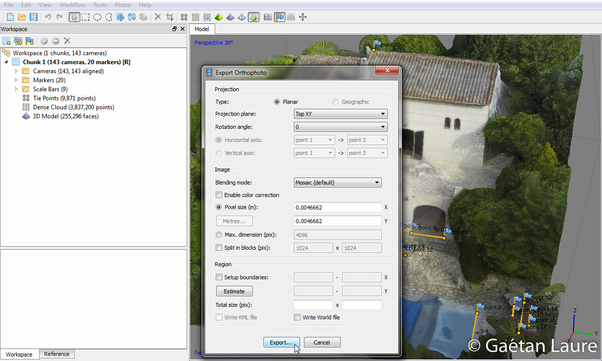
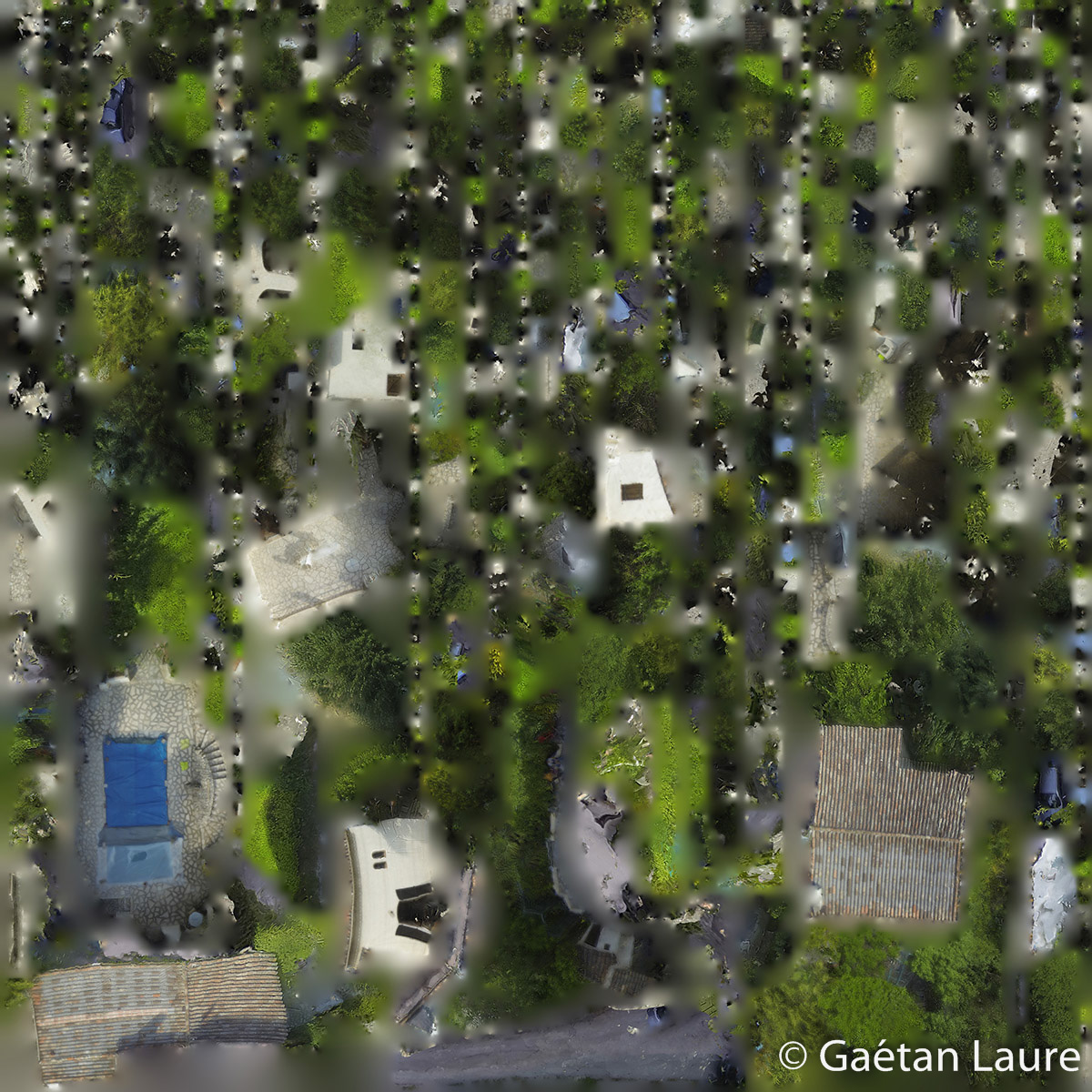
The orthophoto is the projection of the 3D model on a plane. Here I chose the plane XY with a view from the top (X and Y are the axis from the local coordinate system defined using the pool edges). The resolution can be set to a maximum precision of 4.66 mm per pixel.
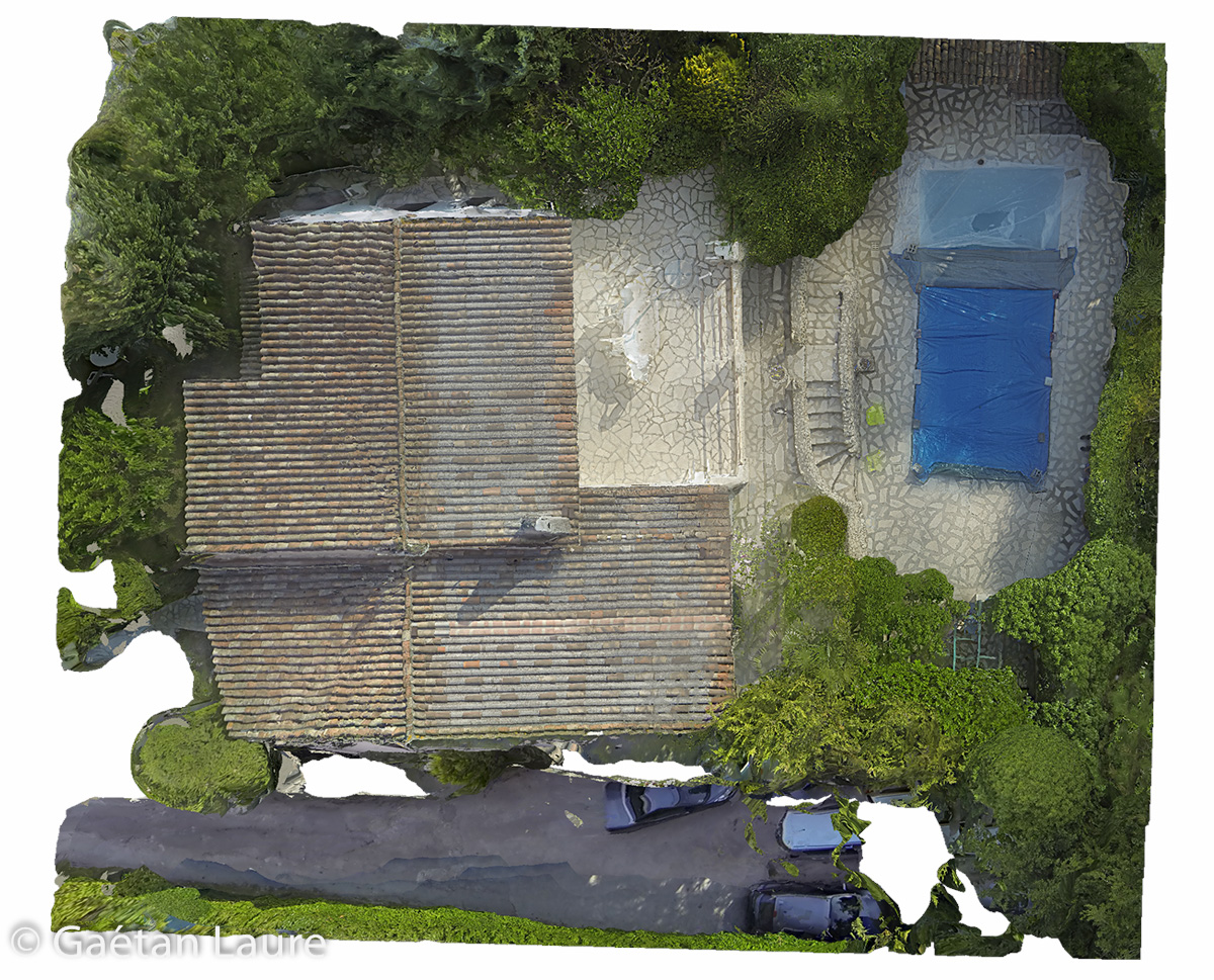
Here is the result (downsized). It’s finally a 2D map built from the 3D model. It’s easy to measure distances because the image has a defined scale.
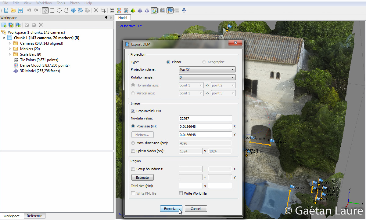
Now let’s compute the DEM (digital elevation model). It provides a 2D image of the elevation of each points relatively to a chosen plane. I again chose the XY plane with a view from the top.
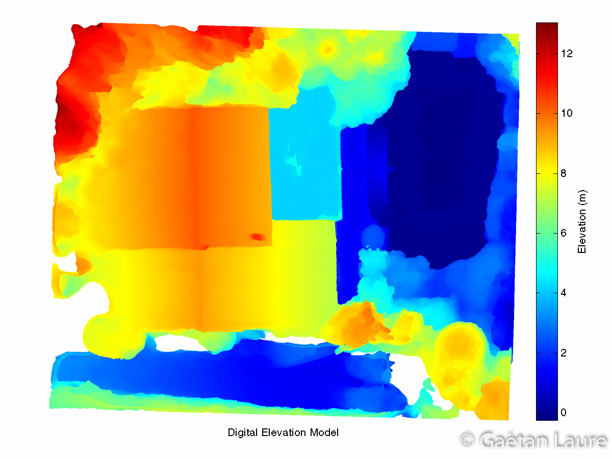
The image exported by PhotoScan is a .tif file. It’s a matrix of floats defining the height (in meters) of each point. I used Matlab to get a colormap from this matrix, display a colorbar and export the result in .png.
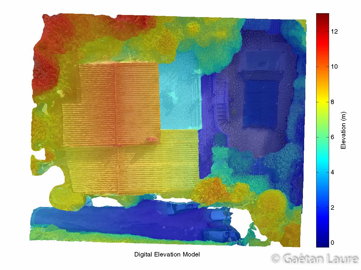
Here is again the DEV merged with the orthophoto. It can be useful to match the elevation with the different parts of the house.
I guess both of these maps can be useful to check quickly the progress of public works for example, measuring horizontal distances and elevations. It can also be used to generate level curves for cartography applications.
Exporting the model in Google Earth
To finish with, let’s show rapidly how we can export the 3D model in Google Earth. The first thing to do is to change the local coordinate system using GPS locations and absolute altitudes to define our reference markers (on the corner of the pool).
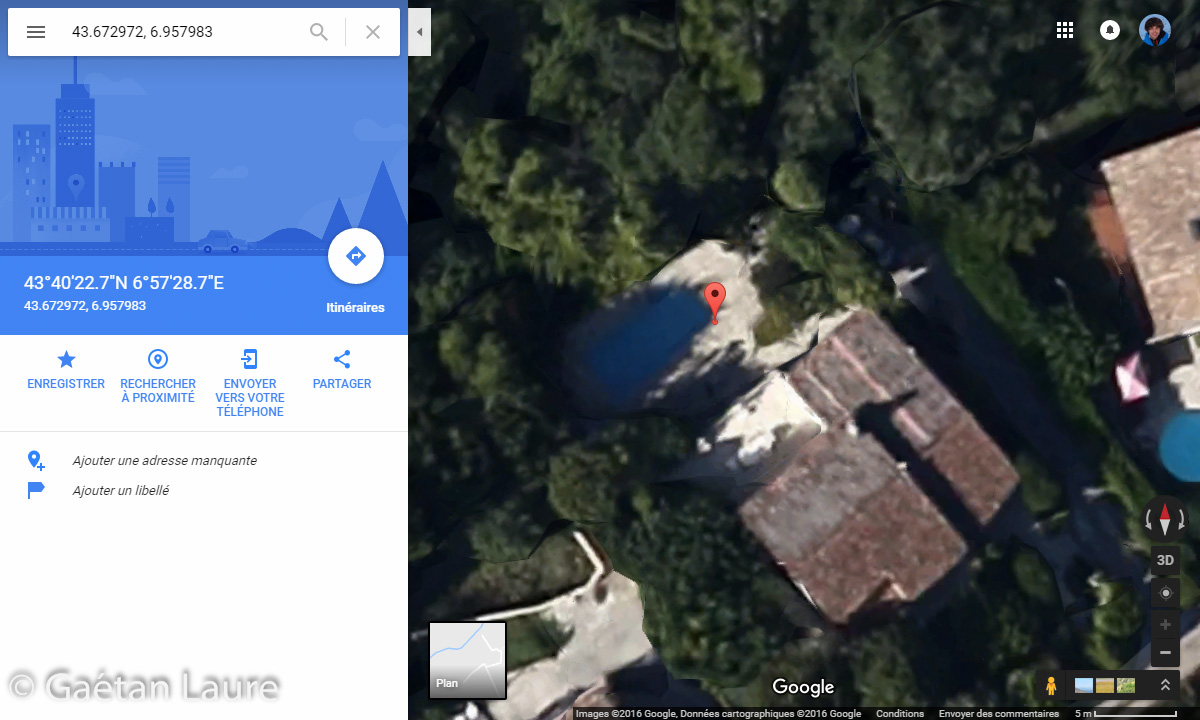
I got the longitude and the latitude of the 3 reference corners of the pool using Google Maps (the same points that I previously used to set the local coordinate system). It’s not the most accurate method due to the resolution of Google Maps in this area. We will see later how to increase the scale calibration of the model.
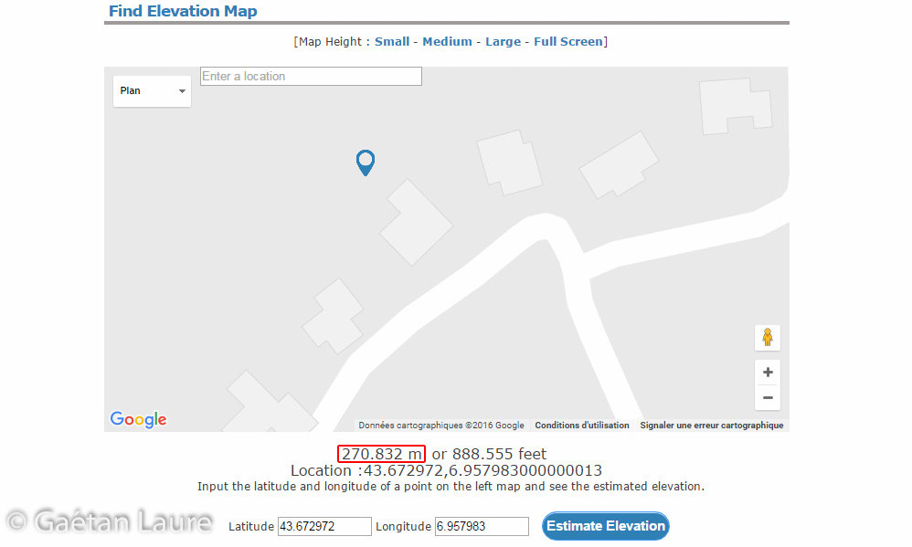
The absolute altitude of these points is known using Elevation Finder site. This altitude has to be corrected to be used in the WGS 84 system adding 49.246 m to it (this value corresponds to the EGM96 geoid altitude correction provided by GeoidEval). The WGS84 altitude of our reference points is then 320.078 m.
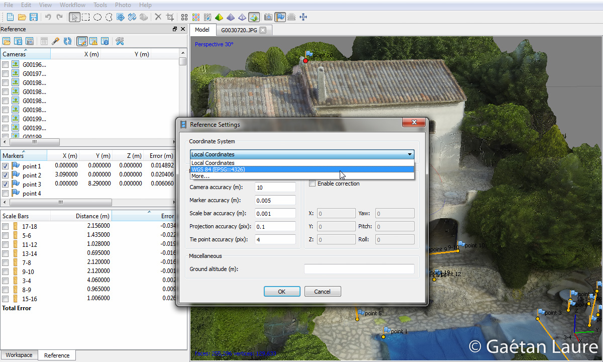
In the reference settings, I set the coordinate system to WGS 84 (EPSG::4326). The 3 reference markers can now be defined using the GPS coordinates.
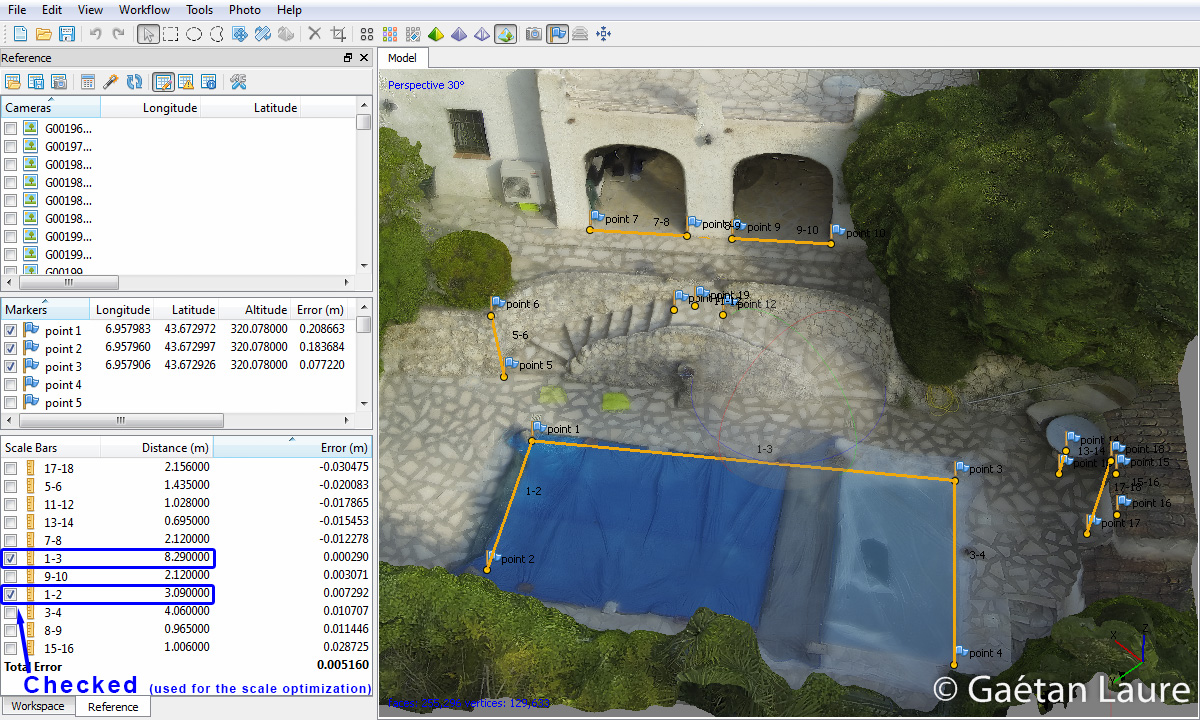
GPS coordinates and altitudes of the reference markers (point 1, 2 and 3) are now set. The GPS coordinates taken from Google Maps for the reference markers aren’t super accurate. This is why I also added two reference scale bars (1-2 and 1-3) corresponding to the sides of the pool between the reference markers. The optimization is then done using the GPS references and the scale bars. After the optimization process, the max error reached is 20 cm for the reference point locations. The maximum distance error (the same 9 distances considered before) is still under 3.5 cm (mean error of 1.87 cm). It means that we keep the same accuracy in measuring distances, areas and volumes in the model (the scale of the model is accurate), but we can’t expect an absolute location of the house in Google Earth more accurate than 20 cm. We can now save the model in .kmz. In this format we will be able to open it in Google Earth.
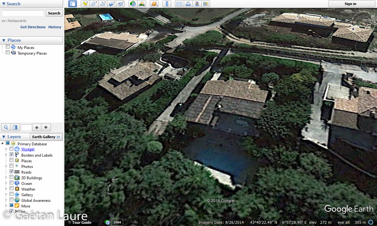
Google Earth before loading the house into it.

Displaying the house into Google Earth. It’s well aligned and oriented and the scale seems consistent. It can be useful to see the reconstruction in its original environment.
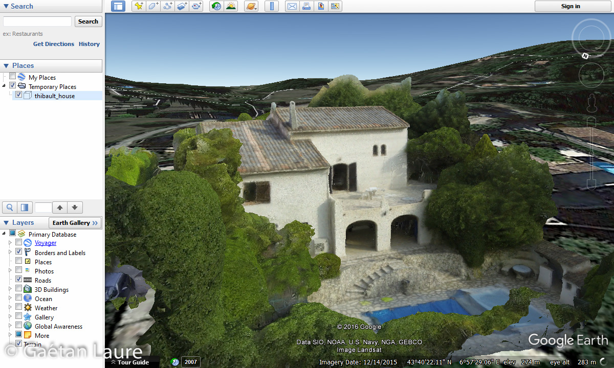
Zooming in.
Conclusion and perspective
In this post, we saw how to perform 3D photogrammetry reconstruction using PhotoScan. It took about 1 hour and 18 mins to process the 3D model (align photos, build dense cloud, build mesh and build texture) with an i7-6700K. I used a GoPro 3 to take the pictures, but it’s not the best camera for this application due to the fisheye lens (with a high distortion). The result is nonetheless quite good, providing an under 3.5 cm precision in the model after having scaled it. We also saw how to build orthophotos and digital elevation models which can be used, for example, in public works, cartography and geology. The model can also be georeferenced and exported into services such as Google Earth to see it in its original environment.
To improve the 3D reconstruction results and get more precision in the model, I should use a camera with a more appropriate lens. The best compromise would be to keep the GoPro which is well suited for use on a drone (small and light, usable with a light gimbal) but replace its lens by a non-fisheye one to increase the accuracy of the reconstruction. Peau Production sells non-fisheye lenses designed to be fitted on the GoPro 3 and 4, such as the 82° HFOV (horizontal field of view) lens or the 60° HFOV lens. These lenses could really improve the result also because of their narrower HFOV (the original GoPro lens has a 123° HFOV) which allow to take smaller area with the same resolution. It will provide more details and information for the 3D reconstruction.
Really nice project and blog post too 😉
Thanks 🙂